Overview This tutorial describes the data reduction for MERLIN 5-GHz radio continuum observations of the radio galaxy 3C277.1. For more information see www.merlin.ac.uk. These data were taken using 6 antennas, Ca (32 m) and Mk Ta Da Kn De, all 25 m. Their sensitivities vary, with De being by far the least efficient at this frequency. The array contains baselines up to 217 km and a usable bandwidth of 13 MHz which has been combined in one channel, hence the data volumne is small and rapid to process (the e-MERLIN upgrade will provide 2 GHz bandwidth). All antennas are alt-az. All four polarizations (RR RR LR RL) are present. Antenna positions are geocentric, terrestrial E, N positive. The data can be downloaded from 3C277.1.MULTTB which is a multi-source file containing: - 3C277.1 (target)
- 1300+580 (phase-reference source and polarization leakage calibrator)
- 3C286 (primary flux scale calibrator and polarization angle calibrator)
- OQ208 (point source flux scale calibrator)
Two flux scale calibrators are used because sources like 3C286 with stable, well-known amplitudes (and in this case polarization) are usually extended over several arcsec or more and hence are heavily resolved by MERLIN. On the other hand, point-like, bright sources like OQ208 are usually variable. Information: If you want to short-circuit any of the steps, or compare your data (see if you can do better!), 3C277.1.FITS is a multi-source file containing target and calibration sources which has already been (mostly) edited. 3C277.1C.SPLIT contains the fully-edited target with all calibration from calibration sources applied, ready for imaging and self-calibration. 3C277.1.CAL.SPLIT is also fully self-calibrated and 3C277.1.FITSIMAGE is the final image in full polarization. These can be loaded into CASA using importuvfits for the first 3 files and importfits for the image. The script below covers: - Loading and inspecting data
- Editing
- Initial phase-calibration of calibration sources
- Setting the flux scale
- Time-dependent amplitude calibration of calibration sources
- Polarization leakage and angle calibration
- Target imaging and self-calibration
- Imaging in polarization
- Image measurements
This script is designed to be used by copying or typing the input to one task at a time, based on the text with a cyan background like this. Further information on any task e.g. importuvfits is obtained from the CASA cookbook or by typing Review the inputs to each task using inp before running it. In some places you have to insert the parameters yourself similar to previous inputs. This script is not intended to run automatically. Import, inspect and flag the data This assumes that all data are in the present working directory; if not, use the path in front of the fitsfile name. Start CASA and set variables for convenience: prefix ='3C277.1C'
msfile = prefix + '.ms'
If you want to delete all data files created here by CASA at any time, type Load the fits data using importuvfits and list the contents using listobs. default importuvfits
vis=msfile
fitsfile='3C277.1.MULTTB'
inp
importuvfits()
listobs()
You see something like this in the logger: ##### Begin Task: listobs #####
listobs::::casa
==============================================================================
MeasurementSet Name: /home/amsr/scratch/ALMA/CASANOTES/3C277.1/3C277.1C.ms MS Version 2
================================================================================
Observer: Project:
Observation: MERLIN2
Data records: 210236 Total integration time = 456357 seconds
Observed from 15-Apr-1995/17:13:58.0 to 20-Apr-1995/23:59:55.0 (UTC)
listobs::ms::summary
ObservationID = 0 ArrayID = 0
Date Timerange (UTC) Scan FldId FieldName nVis Int(s) SpwIds
15-Apr-1995/17:13:58.0 - 17:28:38.0 1 0 3C286 1665 7.99 [0]
17:29:38.0 - 18:29:30.0 2 1 OQ208 6750 7.99 [0]
...
17:07:38.0 - 17:09:54.0 8 10 1300+580 270 7.99 [0]
17:10:37.0 - 17:17:49.0 9 11 3C277.1 825 7.99 [0]
17:18:36.0 - 17:19:56.0 10 10 1300+580 165 7.99 [0]
17:20:35.0 - 17:27:55.0 11 11 3C277.1 840 7.99 [0]
17:28:42.0 - 17:29:54.0 12 10 1300+580 150 7.99 [0]
...
Fields: 7
ID Code Name RA Decl Epoch nVis
0 3C286 13:31:08.2873 +30.30.32.9590 J2000 31538
1 OQ208 14:07:00.3944 +28.27.14.6880 J2000 49583
9 0552+398 05:55:30.8056 +39.48.49.1660 J2000 10560
10 1300+580 13:02:52.4649 +57.48.37.6175 J2000 11785
11 3C277.1 12:52:26.2859 +56.34.19.4882 J2000 60915
12 3C84 03:19:48.1601 +41.30.42.1060 J2000 34230
15 2134+004 21:36:38.5821 +00.41.54.3215 J2000 11625
(nVis = Total number of time/baseline visibilities per field)
Spectral Windows: (1 unique spectral windows and 1 unique polarization setups)
SpwID #Chans Frame Ch1(MHz) ChanWid(kHz)TotBW(kHz) Ref(MHz) Corrs
0 1 TOPO 4994 13000 13000 4994 RR RL LR LL
The SOURCE table is empty: see the FIELD table
Antennas: 6:
ID Name Station Diam. Long. Lat.
0 1 DEFFORD 25.0 m -002.08.35.0 +51.54.50.9
1 2 CAMBRIDG 25.0 m +000.02.19.5 +51.58.50.2
2 3 KNOCKIN 25.0 m -002.59.44.9 +52.36.18.4
3 4 DARNHALL 25.0 m -002.32.03.3 +52.58.18.5
4 5 MK2 25.0 m -002.18.08.9 +53.02.58.7
5 6 TABLEY 25.0 m -002.26.38.3 +53.06.16.2
listobs::::casa
##### End Task: listobs #####
Check the logger. There may be some warnings as CASA does not recognise all FITS extension tables but the vital descriptive information should be present. The target:phase reference source are observed on an 8:2 min cycle. The diameters of all antennas are given as 25 m by default although the Ca dish is 32 m but as the target does not extend far out in the primary beam we can ignor this. Also ignor the spare calibration sources. Plot amplitude as a function of uvdistance to check that the phase reference source is a point (note that plotxy will be replaced by plotms, but at present we use plotxy for convenience in making multiple plots). Right-click on any plot to see it full-size. Inputs to casa are shown over a cyan background. default(plotxy)
vis=msfile
subplot=111
field= '1300+580'
iteration=''
antenna=''
correlation = 'RR LL'
xaxis='uvdist'
yaxis='amp'
inp
plotxy()
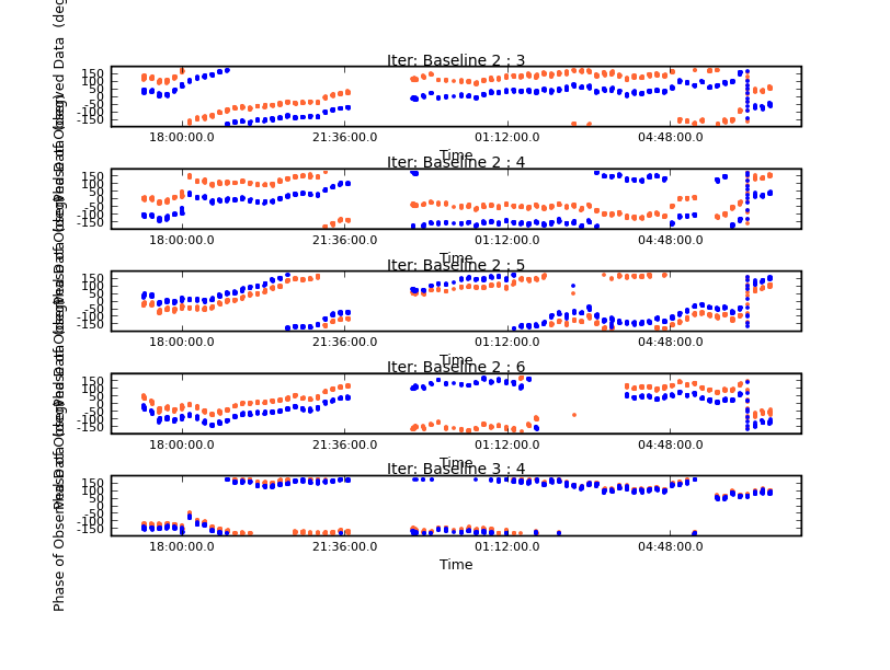
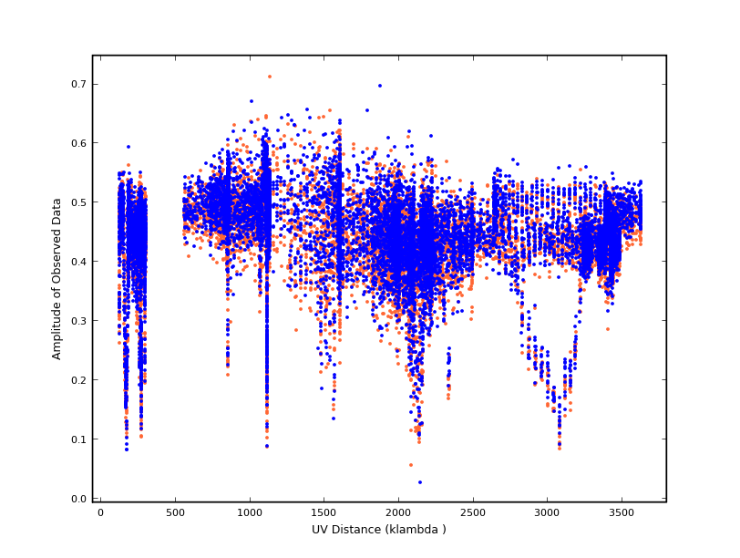 The plot shows some bad data but no systematic trend with uv distance. Antenna '1' (Defford) is less sensitive than the others, so the data are noisier and we will flag by baseline (there are only 15). Inspect the phase reference source and flag the low points of amplitude and the sections where the phase cannot be followed. Use the Next button to iterate through the baselines. xaxis='time'
yaxis='amp'
field= '1300+580'
selectdata=True
antenna = ''
iteration = 'baseline'
subplot = 511
selectdata = True
correlation = 'RR LL'
inp
plotxy()
yaxis='phase'
plotxy()
The phase-reference source amplitudes and phases are shown above. The target is observed in the gaps between each scan. If long periods of data are flagged then there will be no solutions derived for calibration on shorter intervals and the target data in these intervals will normally be flagged also when the calibration is applied. Try a short cut on OQ208 to flag all the data when the source is very low (this takes a little longer, see progress in the logger). field='OQ208'
extendflag=True
extendant='all'
inp
plotxy()
 Some OQ208 baselines after flagging. 3C286 is very resolved, but fortunately it does not seem to need any flagging. We will flag the target 3C277.1 after applying calibration. Back up with flagmanager - add a comment if you like! Use flagmanager any time later if you have done significant flagging. default(flagmanager)
vis=msfile
mode='save'
versionname = msfile+'_calsource.flags'
inp
flagmanager()
Plot the antenna distribution using plotants to chose a reference antenna with good data with many short baselines (easier to calibrate the phase). Ignor messages about not finding the position of MERLIN. I suggest '5' as the refant. 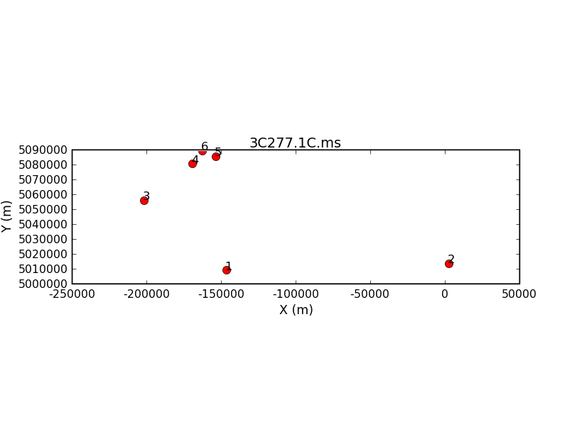 MERLIN antenna positions Setting the flux scale 3C286 is a standard flux and polarization calibration source, with properties tabulated by Baars (1977). It is somewhat resolved even on the shortest MERLIN baselines at 5 GHz, hence a sub-standard flux density used (96% of Baars). It has 11.2% fractional polarization at uvPA 66 deg, which we use to work out Q and U and then insert the values in the MODEL data column of the measurement set using setjy: ipol = 7.073
qpol = 0.112*ipol*cos(66*pi/180.0)
upol = 0.112*ipol*sin(66*pi/180.0)
default('setjy')
vis = msfile
field = '3C286'
fluxdensity=[ipol,qpol,upol,0.0]
inp
setjy()
In order to get enough signal to noise for accurate amplitude solutions we need to average over a few minutes, but the phase changes more rapidly on the long MERLIN baselines. A lower signal to noise is adequate for phase solutions so we solve for phase first with a short solution interval (typically 0.5 min) before deriving amplitude corrections. Both types of calibration are derived using gaincal. default('gaincal')
vis=msfile
caltable=prefix+'_cals.phcal'
field = '3C286,OQ208,1300+580' # No spaces!
solint = '0.5min'
refant='5' # pick antenna with good data near array centre
calmode='p'
minsnr = 3.0
minblperant= 3
inp
gaincal()
Check the logger and plot the solutions: default('plotcal')
caltable=prefix+'_cals.phcal'
field = '1300+580'
subplot = 611
iteration='antenna'
xaxis='time'
yaxis='phase'
plotrange=[-1, -1, -180, 180]
inp
plotcal()
 Phase reference source phase solutions (the range is [-180,+180] deg) Check the solutions for the other calibration sources. Even where the phase solutions are going round quite fast, they should not be random. 3C286 is heavily resolved on the longer baselines so we derive amplitude solutions for it and OQ208 on short baselines only, applying the phase solutions. minsnr=-1 is a fix to allow solutions to be passed on only 3 baselines. vis=msfile
caltable=prefix+'_cals.a1cal'
field='3C286,OQ208'
selectdata=True
uvrange=''
solint='2min'
minblperant =2
minsnr=-1
antenna='4~6&4~6'
gaintable=prefix+'_cals.phcal'
calmode='ap'
inp
gaincal()
Check the solutions, which should be within a few percent of unity. caltable = prefix+'_cals.a1cal'
yaxis='amp'
field='3C286'
antenna = '4,5,6'
plotrange=[-1,-1,-1,-1]
subplot=311
iteration='antenna'
plotcal()
Also check OQ208 - this will have a different mean because there is not yet a proper model. Flag any solutions with a large scatter. fluxscale is used to compare the solutions for OQ208 with those of 3C286 to find the flux density of the former. default('fluxscale')
vis=msfile
caltable=prefix+'_cals.a1cal'
fluxtable=prefix+'_OQ208.flux'
reference='3C286'
transfer='OQ208'
inp
fluxscale()
Note the OQ208 flux density in the logger; the scatter should be less than 1%. I got Flux density for OQ208 in SpW=0 is: 2.3099 +/- 0.00530734 (SNR = 435.226, nAnt= 3)
The fluxtable will contain the proper scaling, but since we have only used a subset of antennas we have to set the flux density of OQ208 (insert your value below) and repeat the amplitude calibration using all antennas: default('setjy')
vis = msfile
field='OQ208'
fluxdensity=[2.31,0]
inp
setjy()
Use this to find the flux density of the phase reference source on all baselines vis=msfile
selectdata=False
field='OQ208,1300+580'
solint = '2min'
uvrange=''
antennas = ''
refant = '5'
minsnr=3
minblperant=4
caltable=prefix+'_cals.a2cal'
gaintable = '3C277.1C_cals.phcal'
inp
gaincal()
Use plotcal to check the solutions (see previously); assuming that they are OK use fluxscale: vis=msfile
caltable=prefix+'_cals.a2cal'
fluxtable=prefix+'_1300+580.flux'
reference='OQ208'
transfer='1300+580'
inp
fluxscale()
Note the flux density of 1300+580 from the logger and set this. This is not strictly necessary as you could simply use the rescaled fluxtable, but it makes accounting easier in later calibration. I got Flux density for 1300+580 in SpW=0 is: 0.425989 +/- 0.000969224 (SNR = 439.515, nAnt= 6)
vis=msfile
field='1300+580'
fluxdensity=[0.426,0]

inp
setjy()
Phase reference source solutions prefix+'_cals.phcal' (i.e. 3C277.1C_cals.phcal) contains phase-only solutions for all the calibration sources including the phase reference source. Make a calibration table for the phase reference source with the amplitude gains correctly scaled with respect to the derived flux density. vis=msfile
caltable=prefix+'_cals.acal'
field='1300+580'
solint = '2min'
uvrange=''
antennas = ''
refant = '5'
minsnr=3
minblperant=4
calmode = 'ap'
gaintable = prefix+'_cals.phcal'
inp
gaincal()
Check in plotcal - the amplitude gains should all be close to unity and the phase solutions should be small since we applied the initial phase calibration table. Note that, unlike AIPS, CASA uses the inverse of the gain correction factors. For example, the points which looked low on antenna 6 in the raw amplitudes, also have low amplitude gains correction factors. 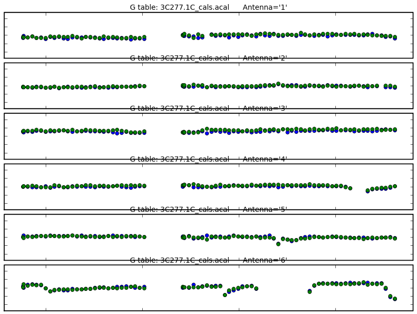 Phase reference source amplitude solutions (the range is [0.5,1.5]). Polarization calibrationThe phase reference source was observed over a wide hour angle range and it is point-like. We can use it to solve simultaneously for its intrinsic polarization and for leakage between the receiver feeds in orthogonal polarizations, using polcal. The parallactic angle correction (to allow for the rotation of alt-az feeds during tracking) is also derived. preavg defines the averaging intervals over which the parallactic angle correction is applied. default('polcal')
vis=msfile
caltable=prefix+'_phref.dcal'
field = '1300+580'
selectdata=False
solint = 'inf'
combine='scan'
preavg=120.0
refant='5'
poltype='D+QU'
minsnr = 3.0
minblperant= 3
gaintable= prefix+'_cals.phcal',prefix+'_cals.acal'
inp
polcal()
Inspect the solutions in the logger or use caltable=prefix+'_phref.dcal'
listcal()
The logger shows polcal Fractional polarization solution for 1300+580 (spw = 0): : Q = 0.0343205, U = -0.01451 (P = 0.0372617, X = -11.4588 deg)
...
polcal Ant=1: R: A=0.04847 P=-19.26 ; L: A=0.04227 P=-90.43
polcal Ant=2: R: A=0.1035 P=-151.6 ; L: A=0.01853 P=-87.4
polcal Ant=3: R: A=0.04337 P=-47.11 ; L: A=0.04684 P=-92.62
polcal Ant=4: R: A=0.026 P=24.81 ; L: A=0.03879 P=-135.4
polcal Ant=5: R: A=0 P=0 ; L: A=0.02193 P=-67.9
polcal Ant=6: R: A=0.04473 P=-121.9 ; L: A=0.01694 P=51.1
The source polarization is expected to be a few percent; I got P/I = 0.0373/0.426 (using the value of P above and the total flux density I from fluxscale). All amplitude (A) solutions should be less than 10% At present, the origin of phase, and hence the polarization angle, is arbitrary. This is corrected using the known polarization angle of 3C286. We apply the phase and polarization leakage solutions and use the model of its I Q U and V previously set. We rely on the amplitude being stable during the short (c. half an hour) observation, to avoid needing to use a model for amplitude calibration, since the polarization is dominated by the compact core. default('polcal')
vis=msfile
caltable=prefix+'3C286.pacal'
field='3C286'
selectdata=False
solint = 'inf' # entire 'combine' intervals = scan length, here.
combine='scan'
preavg=120.0 # interval at which to apply ||actic angle
refant='5' # pick antenna with good data near array centre
gaintable= prefix+'_cals.phcal',prefix+'_phref.dcal'
poltype='X'
inp
polcal()
The polarization angle correction is reported in the logger. polcal Position angle offset solution for 3C286 (spw = 0) = 33.9224 deg.
Apply the calibration and prepare for imagingApply the time-dependent phase and incremental phase plus amplitude solutions to the target and the phase-reference source using applycal. As the MERLIN antennas have different sensitivities we use calwt=False (so that data for the less sensitive antennas are not given too small a weight to be included properly in self-calibration). default('applycal')
vis = msfile
gaintable= prefix+'_cals.phcal',prefix+'_cals.acal',prefix+'_phref.dcal', prefix+'3C286.pacal'
field='1300+580,3C277.1'
calwt=False
parang=True
inp
applycal()
No amplitude calibration table for 3C286: gaintable= prefix+'_cals.phcal',prefix+'_phref.dcal',prefix+'3C286.pacal'
field='3C286'
applycal()
This fills the CORRECTED data column with visibilities multiplied by the various calibration factors. split out the target (further imaging and self-calibration are quicker and simpler using a single-source file): default('split')
vis=msfile
datacolumn = 'corrected'
outputvis='3C277.1C.split.ms'
field='3C277.1'
inp
split()
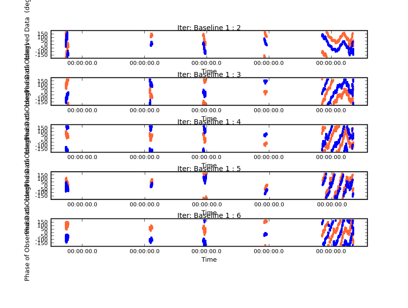
Inspect the calibrated 3C277.1 data. default(plotxy)
vis = '3C277.1C.split.ms'
xaxis='time'
yaxis='amp'
datacolumn='data'
correlation='RR LL'
iteration='baseline'
field = '3C277.1'
subplot=511
plotxy()
 Amplitude and phase of the target after editing Self calibration and imaging of the target Image the target using clean. The longest baseline is 217 km and the wavelength is 6 cm. Use this to estimate the interferometer resolution and hence a suitable pixel size to give at least 3 pixels across the beam. A minimum image size of at least 512 pixels is needed for for adequate deconvolution of the rather extended dirty beam produced by the sparse MERLIN array. psfmode='hogbom' provides a large beam patch for deconvolving extended sidelobes. Note that if interactive=True you have to set box(es) yourself and double click in them to activate. Don't clean too far before self-calibration. Ignor warnings about not finding position of MERLIN default('clean')
cell=['0.015arcsec', '0.015arcsec']
imsize=[512,512]
psfmode='hogbom'
imagermode='csclean'
cyclefactor=4
stokes='I'
interactive=True
niter=1000
gain=0.05
vis='3C277.1C.split.ms'
field='3C277.1'
imagename='3C277.1C_clean1'
interactive=True
stokes='I'
mask=''
inp
clean()
You can save your boxes for future use. In the viewer menu, select Tools > Region in File
Enter Stokes IQUV
Then draw your boxes (you cannot save boxes drawn prior to openning the Region in File dialogue). Click on Save and enter a name, e.g. clean1.rgn. To save the clean inputs for future, use saveinputs saveinputs ('clean', '3C277.1.clean1.saved')
Check progress in the logger. In this instance we have let CASA fit the natural synthesised beam, the size is reported in the logger (and also recorded in the image header). The Clean model is left in the MS in the MODEL_DATA column. Use the viewer to load 3C277.1C_clean1.image as a raster map and use the 'data display options' to tweak it. You can access these via the spanner icon or the Data menu option Ajust. viewer('3C277.1C_clean1.image')
There are several ways to measure the noise and the peak. If you draw a box and double-click, the rms etc. will be displayed. To set the measurement in a variable (here called rms_target) use imstat, setting the limits to avoid the image. default('imstat')
imagename='3C277.1C_clean1.image'
box='20,20,492,120'
stokes='I'
noise_target = imstat()
rms_target=noise_target['rms'][0]
print rms_target
I got 0.00079 Jy. Use the menu Data>Load, select 3C277.1C_clean1.image as a contour image and use the 'data display options' to set the base contour level to the rms_noise and the relative contour levels to [-3,3,6,12,24,48,96].  First image of the target, contours at [-0.0025,0.0025, 0.005, 0.01, 0.02, 0.04, 0.08] Jy/beam You can also overlay the Clean Components (3C277.1C_clean1.model) as a Marker Map using the Data > Open menu (set the x and y increments to 1.) Self-calibrate with gaincal using the model (the Fourier transform of the clean components) left in the MS. It is OK to selfcal in I if V is zero, which is usually the case at all but the highest resolution for extragalactic cm-wave radio continuum. default('gaincal')
vis='3C277.1C.split.ms'
caltable=prefix+'_self1.phcal'
field='3C277.1'
refant='5'
minblperant=3
minsnr=1
calmode='p'
solint = '2min'
parang=True
inp
gaincal()
Check the logger and inspect the solutions caltable=prefix+'_self1.phcal'
xaxis='time'
yaxis='phase'
subplot=611
iteration='antenna'
plotrange = [-1, -1, -180, 180]
plotcal()
You expect to see just residual solutions; if they look OK use applycal.  Target phase solutions (the range is [-180,+180] deg). default('applycal')
vis='3C277.1C.split.ms'
gaintable=prefix+'_self1.phcal'
field='3C277.1'
parang=True
calwt=False
inp
applycal()
Clean, set threshold to the measured noise, rms_target Restore the saved inputs (3C277.1.clean1.saved is just a text file, you can view or edit it) using the python command execfile. If you saved your boxes give the file name as the argument of mask. You can change these interactively in the clean viewer. Restore the previous, saved clean inputs execfile('3C277.1.clean1.saved')
Inspect and adapt the inputs, using the previous noise level as the minimum clean flux. You should stop cleaning when the minimum clean components have sidelobes fainter than the noise. You can calculate the stopping criteria more accurately by inspecting the sidelobe ratio of the dirty beam and comparing that with the expected final noise level. inp
imagename = '3C277.1C_clean2'
threshold=str(rms_target)+'Jy'
niter=2000
mask='clean1.rgn'
clean()
saveinputs ('clean', '3C277.1.clean2.saved')
Make a new region mask if it needs improving. Inspect 3C277.1C_clean2.image as previously in the viewer and check that the noise has gone down. default('imstat')
imagename='3C277.1C_clean2.image'
box='20,20,492,120'
stokes='I'
noise_target = imstat()
rms_target=noise_target['rms'][0]
print rms_target
In this example we go straight to amplitude self-calibration. If the previous phase solutions showed large changes you might do more phase-only calibration first to improve the model, perhaps trying shorter solution intervals and different boxes. Gaincal only works from the original, not corrected data so apply the previous phase self-cal solutions as the gaintable in gaincal. default('gaincal')
vis='3C277.1C.split.ms'
caltable=prefix+'_self2.ampcal'
field='3C277.1'
refant='5'
minsnr=1
calmode = 'ap'
minblperant=4
solint='3min'
gaintable=prefix+'_self1.phcal'
parang=True
inp
gaincal()
Inspect the solutions. caltable=prefix+'_self2.ampcal'
iteration='antenna'
subplot=611
yaxis='amp'
plotrange = [-1, -1, 0.8, 1.2]
plotcal()
The amplitude corrections should be within a few percent of unity. Plot the phase corrections as well, these should be very small residuals. 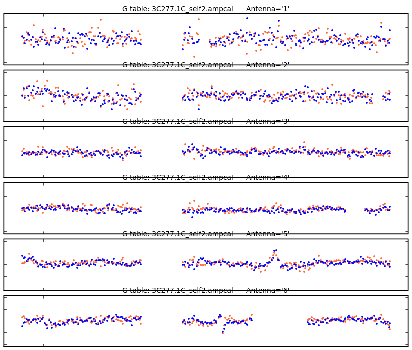 Target amplitude corrections, range [0.8,1.2] Apply both 'p' and 'ap' calibration tables with applycal vis='3C277.1C.split.ms'
gaintable=prefix+'_self1.phcal',prefix+'_self2.ampcal'
calwt=False
parang=True
inp
applycal()
Finally, clean in full polarization. Remember that you can change the threshold or the number of iterations/cycles interactively. If you made a new file of saved clean boxes, update the name of the mask file. execfile('3C277.1.clean2.saved')
inp
imagename = '3C277.1C_clean3'
threshold=str(rms_target)+'Jy'
stokes='IQUV'
niter=5000
clean()
You can use Display Panel options to view all 4 Stokes planes at once. In these settings, the mask is applied to all planes and imagermode='csclean' deconvolved them jointly, which is usually appropriate for small fractional polarization. View and check that the noise has gone down: default('imstat')
imagename='3C277.1C_clean3.image'
box='20,20,492,120'
stokes='I'
noise_target = imstat()
rms_target=noise_target['rms'][0]
print rms_target
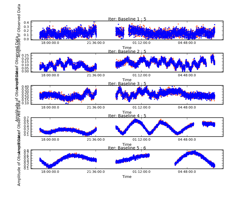
You can check the accuracy of your model by plotting the Fourier transform of the Clean components (in the MODEL data column of the MS) against the CORRECTED visibilities: default('plotxy')
vis='3C277.1C.split.ms'
xaxis='uvdist'
yaxis='amp'
datacolumn='corrected'
selectdata=True
correlation='LL'
field='3C277.1'
timebin='180' # 3 min, same as solution interval
plotcolor='blue'
overplot=true
plotxy()
datacolumn='model'
plotcolor='red'
plotxy()
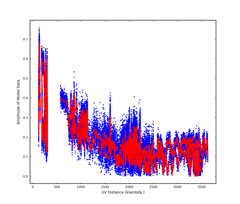 Target model (red) overplotted on the calibrated visibility data. Some scatter in the data is due to real structure below the CC cutoff and to unavoidable noise, which is worse on intermediate baselines because these include Defford, the least sensitive antenna at 5 GHz. If the model is a very poor fit, try more editing and/or self-calibration and/or change the clean inputs Split the total intensity Stokes I image out of final image using immath default('immath')
imagename = '3C277.1C_clean3.image'
mode = 'evalexpr'
stokes = 'I'
outfile = '3C277.1C.icln'
expr='IM0'
inp
immath()
Use the toolkit to make a Q+iU image (needed to plot scaled polarization vectors) potool = casac.homefinder.find_home_by_name('imagepolHome')
pho = potool.create()
pho.open('3C277.1C_clean3.image')
complexlinpolimage = '3C277.1C.cmplxlinpol'
pho.complexlinpol(complexlinpolimage)
pho.close()
Estimate a suitable cutoff for plotting polarization e.g. and note the result Load the I image into the viewer and then use the menu Data>Load to enter '3C277.1C.cmplxlinpol'['3C277.1C.icln'> 0.0024]
in the Load Data LEL expression field, as shown below (change 0.0024 to your value). (DON'T click on anything in the Name list). Click on Vector Map.  How to display scaled polarization vectors from the Q+iU image with a cutoff at about 10-20 times the rms of the Stokes I image. Use Data Display options for the raster and vector images and try adding contours. Compare this with the image made before self-calibration - note that the 3 rms_noise level used as the contour base is now much lower. This plot uses x- and y-increments of 2, debiasing true, amplitude scale factor 2, vector color cyan and contours at: [-0.0004 0.0004 0.0008 0.0016 0.0032 0.0064 0.0128] Jy/beam If time, try to improve the image... More self-calibration, maybe editing, clean more slowly with smaller gain, careful boxing... You could also split out 3C286 and 1300+580 and image these in full polarization as above. There is probably no need for further self calibration of the calibration sources. Anita Richards 19 June 2010
|