| Combining MERLIN and EVN data |
 |
 |
 |
|
Markarian 273 was observed by Bondi et al., 2005 MNRAS 361 748 using MERLIN and the EVN at 5 GHz. We thank Marco Bondi et al. for kindly providing the data. Knappen et al. (1997) published a MERLIN-only 5-GHz image which shows that the detectable emission lies within a 2-arcsec region; if planning observations you should check how much you can average the date to avoid bandwidth smearing. The EVN data have baselines up to 2500 km, more than ten times the longest MERLIN baseline between Cambridge and Lovell; this baseline was included in both arrays. Estimate the maximum uv distance present in the data, in kilo-lambda (answer lower down). The data were correlated separately and the individual data sets were calibrated using the same sources including the phase reference source J1337+550, which was observed at the same position for both data sets (you should check this for other data). After applying the calibration, the target (which is too faint to self-calibrate) was split out. The data must have compatible spectral configurations; in this case both data sets have been averaged to a single channel. The data sets are fully calibrated and edited; we only have to combine them. MKN273_EVN.UVDATA MKN273_MER.UVDATA The naturally-weighted MERLIN-only map has a beam size of ~50 mas; the EVN-only map has a beam size of ~10 mas and is insensitive to emission on scales >60 mas. The beam size ratio of 1:25 (EVN : MERLIN) means that a lowest contour at the same flux density in Jy/beam corresponds to a brightness temperature 25x higher in the EVN image. In fact, the rms is slightly lower in the EVN image (as the collecting area is larger) but still only the brightest hot-spots are detected. This example illustrates:
Load and assess the dataThis assumes that settings not specified are default; use RESTORE 0 if necessary before starting. Check all settings with INP before running each task.Load the files into AIPS with FITLD task 'FITLD'This should show two files, MKN273_EVN .UVDATAthe first being the calibrated EVN uv data, and the second the MERLIN data. Use IMHEAD to check the frequencies and positions in the headers. In this case, the positions are identical and the frequencies are close enough that there will be no detectable spectral index effects. The Observ. date is also identical. However, the EVN data are only in dual polarization. You can examine the data using UVPLT. The plot limits are set to the longest uv distance present in the data, 2500,000/0.06 (max. baseline/wavelength) converted to kilo-lambda. TVINIWait for the plot to finish INN 'MKN273_MER';INCL 'UVDATA';INSE 1
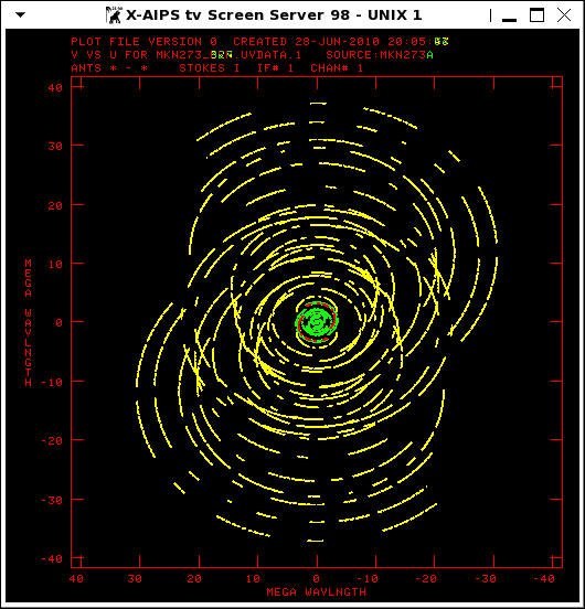 EVN baselines are shown in yellow and MERLIN in green; the overlap on the Cambridge-Lovell baseline shows up in red. Correcting the amplitude scaleEven though the data sets were taken contemporaneously the amplitude scales were set separately; for MERLIN using 3C286 and for the EVN using Tsys measurements. These data were taken with the Cambridge and Lovell telescopes in both arrays, so we can check the amplitude scale by comparing the amplitudes on their baselines.Use PRTAN to identify the antenna numbers of Cambridge (called CM in the EVN data) and Lovell (called JB in the EVN data). task 'PRTAN'This allows us to compare the apparent flux densities on the same baseline lengths, binned for clarity. The maximum length of the baseline is 217000/0.06 lambda; the actual range covered is slightly less than this due to elevation effects TVINI  The EVN data appear to be about 25% brighter than the MERLIN data. INN 'MKN273_MER';INCL 'UVDATA';INSE 1This shows that a flux density of 2.514 Jy was used for OQ208. MERLIN flux measurements show that this is a typical or slightly high value for OQ208 at this frequency, so probably the EVN data have the flux scale set too high, which is possible because the Tsys method was not totally reliable when the observations were made, more than 5 years ago. Repeat UVPL with the data averaged to a single bin per data set and note the Y values reported in the Message Server. TVINII got EVNThe Y values are the mean flux densities for the EVN and MERLIN data on the Lovell-Cambridge baseline. We multiply the EVN data to be consistent with the MERLIN flux scale (use your values here). task 'UVMOD'Type PCAT to see the new file, MKN273_EVN .UVMOD. Run UVPLT again using this file to check that the flux densities are now almost the same. Weighting, combining and imagingThe maximum EVN baseline of about 40 Mlambda implies a full resolution around 6 mas and so a pixel scale of 1.5 mas is needed to provide more than 3 pixels across the beam. In turn, this implies an image size of 2048 pixels to cover a 2-arcsec field. For MERLIN-only, 15 mas is usual (work out why from the maximum MERLIN baseline). Make test images (natural weighting) for both data sets (MKN273_MER.UVMOD.1; MKN273_EVN.UVDATA.1). First, use the rescaled EVN data, total intensity, natural weighting. Box the emission which is visible and stop cleaning when it all looks like noise. Repeat for the MERLIN data, with appropriate cell and image sizes.task 'IMAGR'Note the weights in the messages as each IMAGR starts; I got: EVNThese are in a ratio of about 1:500 EVN:MERLIN (check for yourself) so, to produce a combined data set with equal contributions, the inverse of this is used. DBCON is used to combine the data sets. DOPOS 1,0 is used because the position but not the frequency agree exactly. DOARRAY -1 is used because the arrays are different so both antenna tables will be copied. task 'DBCON'You should now see M273_ME_.002. DBCON (the name was chosen to remind me of the combined proportions). Image the combined data. Use the pixel size needed for the longest baselines present. tget IMAGRInspect the header of the output image and note the Maximum and the fitted beam size, termed Conv size. Display the image. PCATTVPSEU and TVZOOM can be used to change the colour table and to zoom. Use TVWIN to select an off-source region and IMSTAT to measure the noise statistics Compare with the EVN and MERLIN images alone, e.g. Array Beam (mas) Peak (mJy/bm) RMS (mJy/bm) Experiment with different weightings (values of ROBUST) in IMAGR. To improve the sensitivity to extended emission, give MERLIN a higher weight in DBCON, e.g. REWEIGHT 1 0.01. You can write the FITS data to disk using FITTP; you could even load the combined uv data into CASA and experiment with the imaging options there. To exit AIPS, type KLEENEX. 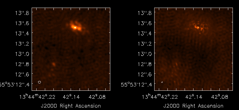 The left hand image has the MERLIN and EVN data combined in proportion 1:1; in the right hand image the proportions are 1:500. |