| VLBI calibration |
 |
 |
 |
AuthorsMarc Ribo, largely based on the 2009 ERIS example, originally from Bourke (with Baan, Beswick, Venturi), with comments from Javier Moldon. Here with Katherine Blundell, Elmar Koerding, James Miller-Jones, Anita M.S. Richards. Assumptions 1. Katherine Blundell: imaging and self-calibration. General scheme Prepared data: N09L2, an EVN Network Monitoring experiment.
Overview
This tutorial concentrates on the analysis of an EVN (European VLBI Network) observation. For more information see www.evlbi.org. The observation consists of about a 2-hour phase referenced portion switching between 4C39.25 (the calibrator) and J0916+3854 (the target source). In the second half of the observation, five bright sources are observed. These data were taken at 1.6 GHz using 10 antennas with very different sensitivities. We will see more details as we proceed. You can also access the JIVE (Joint Institute for VLBI in Europe) archive web page of these observations at http://archive.jive.nl/scripts/arch.php?exp=N09L2_090602. The data are available here n09l2_1_1.IDI. Ancilliary files are n09l2.antab.gz and n09l2.uvflg. This tutorial is in AIPS. This script is designed to be used by copying or typing the input to one task at a time, based on the text with a cyan background like this. Further information on any task, e.g., FITLD is obtained from the AIPS cookbook or by typing help fitld explain fitld Review the inputs to each task using inp before running it. Loading the dataGo to the directory where you placed the files n09l2_1_1.IDI, n09l2.antab.gz, and n09l2.uvflg. Uncompress what is needed (gunzip n09l2.antab.gz). Start aips by typing:
aips tv=local Select a new user ID number, like 200:
200 Three new windows should have been opened: AIPSTV, AIPS-MSGSRV and AIPS-TEKSRV. To start from default values type:
restore 0 Use the task FITLD to load the data. To see the current inputs you can type 'inp'. To see more details about the task and inputs you can type 'help fitld'. To read all details about the task and inputs just type 'explain fitld'. This applies to all tasks.
default fitld You see something like this in the window where you are typing (you have to press RETURN a few times): >inp And now you can type the parameters:
datain 'PWD:n09l2_1_1.IDI Note that there is no closing quote ' after the file name. This means AIPS will keep the case in the string (normally it converts to upper case). We also give an outname to make it more clear that the data refer to the experiment N0912. The CLINT parameter defines the time interval between entries in the calibration tables. Setting this to a lower value (default is 1 minute) will allow us to calibrate on lower time scales later in the process (assuming we have good enough signal to noise). We'll set it to to 1/3 (20 seconds). VLBI datasets are often quite large (many GBs), setting DOUVCOMP = 1 saves disk space. In The AIPS_MSGSRV_1 window a text like this will appear: LOCALH> FITLD1: Task FITLD (release of 31DEC10) begins Now type pcat to check that the file is there:
pcat and you should see: >pcatThe assigned catalog number is 2. This means that any file that we create now will be 1, and then 3, and so on. To avoid this mess, we just type:
recat Now we can type again:
pcat and see that now it reads: >pcatNow we pick up the file and look at the fits header (or "image header"):
getn 1 getn 1 sets INNAME, INCLASS, INSEQ to the values of dataset 1 in the catalog (as seen when you 'pcat'). You should see something like this: >imh First realize that this was already shown at the end of the AIPS_MSGSRV_1 after FITLD. We can see it has 4 stokes parameters, 4 sub bands (AIPS calls these IFs) and 16 channels per sub band. As the data contains many sources the RA and DEC will either contain the coordinates of one of the sources in the data or may be 00. Note that since we have and NX table, we don't need to use INDXR. The data is in Sort order TB (Time Baseline), so everything should work without applying any additional initial tasks. The tasks LISTR and PRTAN can be used to generate a scan listing, and an antenna listing respectively.
default listr The default value of 'docrt' is 132. This will cause the listing to be displayed in your terminal. Using docrt -1 allows you to send it to the printer or to a file. Using docrt -3 avoids anoying carriage returns and page limits. Then you can inspect the scans available in this fits file by going to the corresponding directory and typing 'more scans.txt'. There you will find the scans numbered, with initial and final observation times, together with a list of sources with corresponding positions and the frequencies used. It looks like this: File = N0912 .UVDATA. 1 Vol = 1 Userid = 2234You can see that there are 7 sources observed from 12:30 to 17:30, including 4C39.25 (the calibrator) and J0916+3854 (the target), together with five other sources: 3C84, 3C273B, 3C286, OQ208, and 3C345. You can also see the frequencies of the 4 IFs, which have a bandwidth of 8000 kHz, or 8 MHz, each (32 MHz in total). Since we have 16 channels per IF, the separation between channels is 500 kHz. And now the antenna listing:
default prtan Ant 1 = CM BX= 979610.5344 BY= -1423711.9857 BZ= 375158.5618An issue is the possibility to include the ionospheric corrections. This has to be done at the beginning for the VLBA, and can also be done for the EVN in phase referencing experiments at low elevations. However, the improvement for the EVN has not yet been tested, so we will not apply these corrections here. Interlude: plotsTo get a feeling for interferometry, plotting the data, and calibration tables is important. Any plot will create a plot table (PL) by default unless you specify dotv 1, in which case the plot will be shown in the AIPSTV window. PL files are useful when you want to export a plot as a postscript file. The task LWPLA exports postscript. Useful plots: - UVPLT can display your visibilities. You can specify what the axes represent. Default is amplitude vs uv-distance. Type 'explain uvplt' (after setting docrt 132) and look at the bparm value to see what can be on the axes. - POSSM will plot your amplitudes for each baseline as a function of frequency. - VPLOT can plot each baseline, amplitude or phase, etc., as a function of time, optionally averaging channels. SNPLT can plot your solution (SN) and calibration (CL) tables. It is important to look at the calibration tables after a calibration task. Look out for large (suspicious) jumps in amplitude and phase. When plotting uv data, if the datasets are large, plotting can take a long time. The 'xinc' parameter can be set to skip data, e.g., xinc 10 will plot every tenth point. timerang specifies a limited time range to plot. The format is startday, starthour, startminute, startsecond, endday, endhour, endminute, endsecond. "timerang 0 13 0 0 0 13 5 0" would select five minutes of data from 13:00 to 13:05 on the first day. Type this:
tvin The AIPSTV window should display this after a while (plot #1): 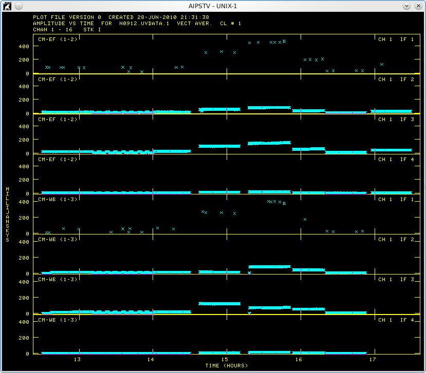 Here you see the amplitudes as a function of time for each IF in each baseline. Hit TV button A to pause indefinitely. Hit button B or C to continue sooner, button D to stop plotting.
tvin The AIPSTV window should display this (plot #2): 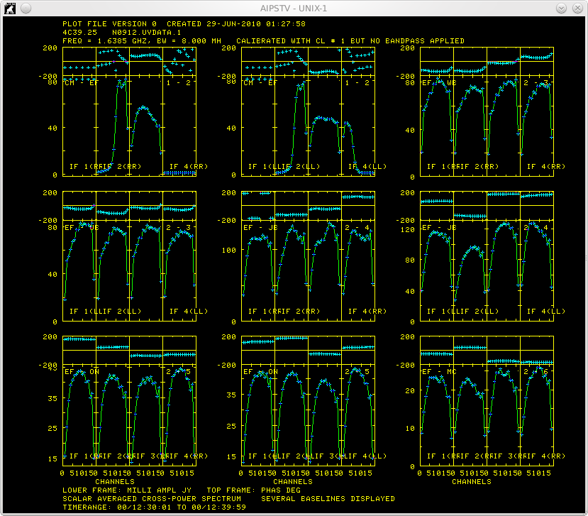 Here you see the phases and amplitudes as a function of frequency channel for each IF in each baseline. Note that CM has a limited bandwidth of about 16 MHz. Note calibration issues at the border channels in each IF, in particular the drops in the amplitude. It is clear that there are "phase jumps" between IFs, and that there are phase drifts within each IF. We will correct for those.
tvin The AIPSTV window should display this (plot #3):  We only plot one point every hundred points, and this already takes about 30 seconds... If you did not specify xinc you should stop the execution. To do this just type "abort" and afterwards "clrstat" (to clean the reading status of the file). As you can see, there are baselines up to 45 Mlambda, meaning that the beam size will be of around 2.2e-08 radians, or 4.6 mas. When imaging, we will select a cellsize of 1 mas. Applying external flag tablesFlag tables are provided with the data. These are generated by the scheduling program at the observatory, and by the observation stations during the observation. Flag tables are useful to flag the times when each dish is not on target due to slewing, source set, etc. These can be attached to the dataset with the task UVFLG.
default uvflg If you type "imh" you will see that now there is a flag table FG. You can further inspect the data for the calibrators and flag what you think is 'strange', particularly for the compact sources. We will not do this here. Amplitude calibrationNow we will modify the original visibility amplitudes to convert them into real flux densities of the sources. This correction involves a scaling factor for each IF in each antenna. To use an astronomical source for amplitude calibration it must meet certain criteria; it must be relatively near to the target in the sky, have quite high flux, be reasonably compact and have a well known source model at the resolution of the instrument. Such sources are rare at VLBI resolutions and so another means of amplitude calibration is required. To accomplish this the antennas have an electronic noise source incorporated into them which is briefly triggered many times throughout the observation to allow the measurement of the system temperature of the antenna. This is done at the observatories and the results are provided to the astronomer as an 'antab' file. This is attached to the data with the task ANTAB. Also present in the file are the Gain Curves for each antenna. These relate the gain of the antenna as a function of elevation angle. AIPS can then use this information to determine amplitude calibration values for the observation.
default antab If you type "imh" you will see that now there is a Gain Curve table GC and a Tsys table TY. The task APCAL is used to generate a solution table SN of amplitude corrections from the Tsys (TY) and Gain Curve (GC) tables.
default apcal If you type "imh" you will see that now there is a solution table SN. We can inspect the content of this table by typing:
tvin The AIPSTV window should display this after you type B once (plot #4):  Here you see the amplitude solutions that should be applied to Effelsberg. Some editing to delete bad points could be done.
default clcal This creates a new calibration table CL 2 (check by typing "imh"), which contains the values from CL 1 (which had constant values, amp 1, phase 0, created by FITLD while loading the data) and the solutions from SN 1. By default CLCAL will use the highest CL table, and all SN tables. This is ok now, as we have only 1 SN table, however we should be careful in future to specify which SN tables to use as we don't want to re-apply a SN table that has already been applied. SNVER = 1 would mean only SN 1 would be applied. Parallactic Angle correctionWe can use the utility vlbapang to correct for parallactic angle effects. It is provided with aips in the vlbautil script. To use it do:
run vlbautil Phase calibrationPhase calibration is slightly more complicated at VLBI scales than at EVLA scales, as the positions of the antennas can be slightly different than what the correlator thought they were. Also, each antenna uses its own clock, so the times can be slightly different at each station, and the times can drift relative to each other. These errors are very small but cause the phases to vary with frequency. The task FRING is similar to CALIB but will solve for the delays (phase slopes with frequency) and rates (phase slopes with time), as well as the phases. A strong point-like calibrator is needed to solve these parameters. It can be useful to first solve for delays only with a short piece of timerange on a bright calibrator, and then solve for all parameters with all calibrators using the delay-corrected data (which also corrects for the phase jumps between IFs). To see the effects of FRING we will look at 2 minutes of the strong calibrator 4C39.25 first by typing:
tvin The AIPSTV window should display this (plot #5): 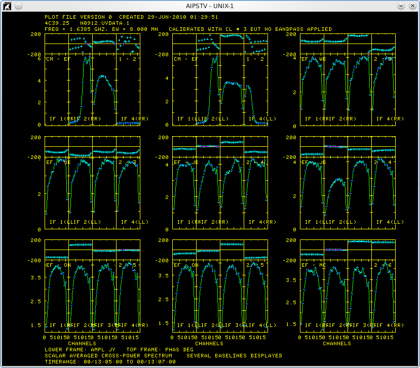 In general, there is a phase slope across each IF, as well as a phase offset between IFs. These instrumental offsets between IFs can be corrected with the delay calibration for a short period (2 minutes or less) of a bright calibrator. We will do this now.
default fring We chose 2 minutes of the strong calibrator 4C39.25. For the reference antenna it is better to chose a big one that is always observing: Effelsberg. The default solution interval is 10 minutes, but we specified only 2 minutes with timerange, so it is ok. DPARMs include gory details... This creates SN table 2. We will apply these delay corrections with CLCAL:
default clcal This creates table CL 4 after applying SN 2 solutions to table CL 3. And now we look with POSSM again:
tvin The AIPSTV window should display this (plot #6):  It is clear that we have corrected for the delays, since all phases look flat for this scan.
tvin The AIPSTV window should display this (plot #7):  As it can be seen, the phases are flat, but different from zero except for the scan that we used to do the initial fring. This is because we have not still corrected for the rates.
default fring LOCALH> FRING1: Found 7930 good solutionsFailing at 10% of the solutions is not critical. Everything went ok. FRING has created table SN 3. We apply these calibrations to create a new CL table, based on the calibrator sources and applied to all sources:
default clcal This creates table CL 5 after applying SN 3 solutions to table CL 4. CLCAL interpolates the solutions which were calculated by CALIB or FRING. It will interpolate the calibration solutions for the calibrator source to the target source. When we last ran CALIB/FRING we requested solutions every 2 minutes (solint 2) now these will be interpolated to the CL interval (20 seconds - set when we did FITLD). Here we have requested that all sources be calibrated. The interpolation mode 'ambg' is useful with FRING calibration. And now we look with POSSM again starting from the first scan:
tvin The AIPSTV window should display this (plot #8): 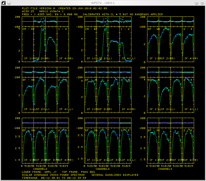 As it can be seen, the phases are flat and zero for all scans (keep typing B on the AIPSTV screen). We can check if this is also the case for the target source:
tvin The AIPSTV window should display this (plot #9):  The phases are flat in all cases, and also zero in most cases. However, for long baselines (EF-SH) this is not the case. This probably means that the source has intrinsic structure. (Moreover, if the source position was not properly known, and hence not located at the correlated phase center, now the phases would not be zero even for a point-like source). Bandpass calibrationWe will calibrate the gain response across our bands (for amplitude and phase) using the task BPASS with the source 4C39.25:
default bpass This creates a bandpass table BP 1. To see the effects of this we should use now the following parameters when appropriate "doband 1" and "bpver 1". And now we look with POSSM again at the 2 minutes of 4C39.25 originally used to solve for the delays:
tvin The AIPSTV window should display this (plot #10):  Phases and amplitudes are nearly flat within each IF. Apart from CM, phases are nearly flat along all the spectrum. Amplitudes vary slightly from IF to IF, but this is normal. We can now apply all calibrations and start mapping. Splitting the dataWe will now create separate datasets for each source with all the flags, and calibrations applied:
default split Setting aparm(1)=1 and nchav causes the channels to be averaged together - this is ok only after you have fring fitted the data. We now have many single source datasets. Type pcat and you should see: >pcatWe can image these as in the other tutorials, e.g., for the target source:
default imagr Afterwards you have to do recat:
recat
default imstat To do self calibration you should use CALIB, for example with the original data and the clean components of the image you have just obtained:
default calib LOCALH> CALIB1: Writing SN table 1It is ok (my rule of thumb, if failed on less than 10% solutions it is ok). Now you should do the image of the new file obtained with CALIB:
tget imagr
recat
default imstat The source is point-like at this stage. We stop here in this tutorial. Further issuesIn general, VLBI arrays contain a few antennas, and the UV-coverage is sparse. Having less baselines makes the self-calibration more difficult, as we have less redundancy. Usually, the source model obtained with the first self-calibration is not perfect, and can be improved. A common procedure is to make several self-calibrations using better models each time, for example doing two phase calibrations (to get an initial good model) and then solve for amplitude and phase (solmode='A&P'). Depending on the quality of the calibrator, it could be needed to use long solution interval for the first amplitude self-calibration (even the full observation). In that case, you can repeat the three P, P, A&P calibrations again with a shorter solution interval for the A&P step, for example one third of the initial one. Proceed iteratively until you reach a phase and amplitude calibration of a few minutes. Stop if the number of bad solutions increases too much. A good point to stop is when the noise of your image is not reducing anymore. It is better to end up with a phase-only self-calibration. You can also plot and edit the clean components (CC) after each imaging step with CCNTR and CCEDT, to apply only those CC that are coming from the source. During this process you have to keep checking the phases and amplitudes as a function of uv distance. For precise astrometry, it can be useful to set an input model when doing FRING, including a good self-calibrated image of your calibrator. Still room for improvement, but this is the general idea. All sorts of schemes for imaging are possible at this stage: you are entering the black belt (and obscure) VLBI area... Marc Ribo, 30 June 2010 |