This tutorial works through an example use of the CASA simdata task. It was originally developed by Ian Heywood (Oxford). For this example, we use CO_CLUSTER.FITS.gz. This shows a cluster of galaxies from the S^3-SAX simulation generator (Obreschow et al. 2009) in the 12CO J(2-1) transition, rest frame frequency 230 GHz, at redshift 1.351, which puts it into ALMA band 3 (around 90 GHz).

The inputs are a model FITS image of CO from a high-redshift galaxy, and an antenna table corresponding to a chosen array (ALMA early science).

The outputs are simulated visibility measurement sets with and without added noise, and the image as it would look like when observed using the chosen array, i.e. sampled by the antennas in the positions supplied over the time interval specified.

Obtaining the simulated data and antenna table

Model antenna tables are provided within the CASA installation. These are examples of how to find the model antenna tables; it may be different for different CASA releases or operation systems.

/home/amsr/CASA/casapy-30.1.11097-001/

/data/alma/simmos/alma*.cfg

/Applications/CASA.app/Contents/data/alma/simmos/

We will use

alma.early.large.cfg 

which is for 16 antennas, baselinesup to c. 1 km, typical of early science. It is a plain text file so you can inspect it using more or a text editor.

Prospective locations of antenna pads, in blue, (left) and visibility plane coverage (right) for ALMA early science in the extended configuration.

This script provides sample inputs for simdata, which takes a model image or datacube, and produces a measurement set sampled using a given set of ALMA antenna locations, observation duration etc.

The data are then used to produce a cleaned image cube. For convenience, assign a variable to the name you want to call the output data e.g.

outsimname = 'COsim'

COsim.noisy.ms       # the measurement set generated using                 
                     # 'observational' parameters including atmospheric noise
COsim.clean.image    # the cleaned datacube

help 'simdata' 

The script below assumes that CO_CLUSTER.FITS and alma.early.large.cfg are in the present working directory.

Inputs to simdata

Start CASA, and inspect the inputs to simdata:

default simdata

inp simdata 

Sky Setup

modelimage   = 'CO_CLUSTER.FITS'
ignorecoord  = True

Observation Setup

project can be set to any name you like. The values for the parameters below that are suitable for these data, but you can experiment with different values. There will be limited ALMA configurations for early science.

noise_thermal = True uses an estimate of the noise likely to result from the chosen observing parameters.

These inputs control the output measurement set properties

antennalist  = 'alma.early.large.cfg' 
project      = outsimname                
refdate      = '2012/05/21/22:05:00'
totaltime    = '7200s'
integration  = '30s'
startfreq    = '89GHz'
chanwidth    = '10MHz'
nchan        = 32
direction    = ['J2000 19h00m00 -40d00m00']
noise_thermal = True                

Imaging Parameters

cell         = '0.02arcsec'
imsize       = [256,256]
niter        = 2000
psfmode='hogbom'

inp

The other inputs are not used in this simple example (they allow you to add phase-reference interruptions, to prepare a mosaic and so on).

Check these inputs and run the task if all looks right.

go simdata

simdata Output

While simdata is running, the logger reports the parameters used to calculate the thermal noise and other progress. Note that there is not any other, systematic atmospheric corruption of the phase nor amplitude absorption. The output will be equivalent to data which have already been well-calibrated.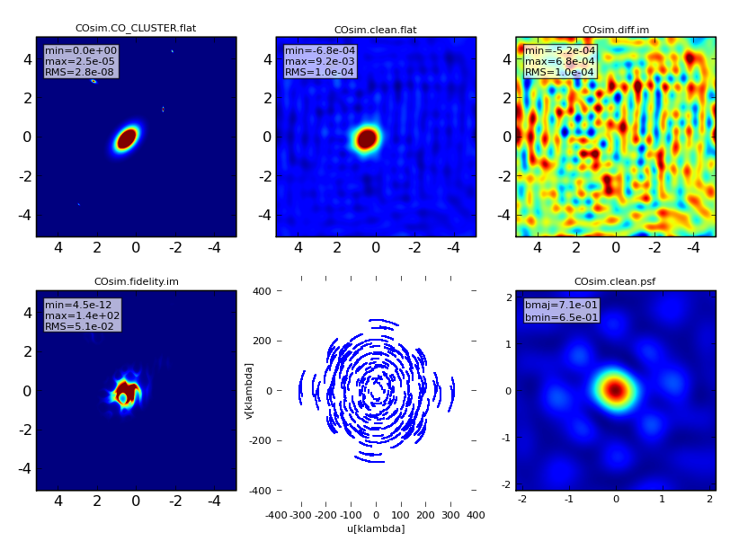

When the task has finished, you should see a display window like this. COsim.clean.flat is a zeroth moment, i.e. emission summed over all planes of the cubes. See Dirk's talk for an explanation of the fidelity image.

A listing should show new subdirectories including:

ls

COsim.clean.image
COsim.noisy.ms

Use the viewer animation controls to display all the planes of the cube. Use the Image Profile tool from the Tool menu.

viewer(outsimname+'.clean.image')

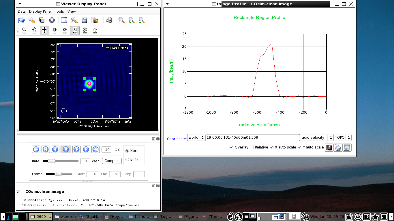The spectrum on the right is derived from the area enclosed in the box on the left-hand image.

default('imstat')
imagename=outsimname+'.clean.image'
box='21,21,230,80'
stokes='I'
noise_target = imstat()
rms_target=noise_target['rms'][0]
print rms_target

Make the first moment (flux-weighted velocity). Use about 7*rms_target as the noise cutoff (the first parameter value for includepix) - insert your own value instead of 0.005. The second value, the upper limit, is usually some arbitrarly large value.

default(immoments)
imagename=outsimname+'.clean.image'
moments= 1
axis= 'spectral'
includepix= [0.005, 200.0]
outfile=outsimname+'.clean.image.mom1'

inp
immoments

viewer(outsimname+'.clean.image.mom1')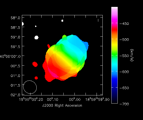

The flux-weighted velocity (first moment) of the simulated image cube.

If you like, you can try different clean parameters on the measurement set produced, COsim.noisy.ms.